Visualising the change in a response variable between two points in the simplex space

The helper function for plotting the change in a response variable over a straight line between two points across the simplex space. The output of the simplex_path_data function (with any desired modifications) should be passed here. The generated plot will show individual curves indicating the variation in the response between the points. `Pie-glyphs` are used to highlight the compositions of the starting, ending and midpoint of the straight line between the two points.

Usage

simplex_path_plot(
  data,
  prop = NULL,
  pie_positions = c(0, 0.5, 1),
  pie_radius = 0.3,
  pie_colours = NULL,
  se = FALSE,
  facet_var = NULL,
  nrow = 0,
  ncol = 0
)

Arguments

data: A data frame created using the simplex_path_data function.
prop: A vector of column names or indices identifying the columns containing the species proportions in the data. Will be inferred from the data if it is created using the `simplex_path_data` function, but the user also has the flexibility of manually specifying the values.
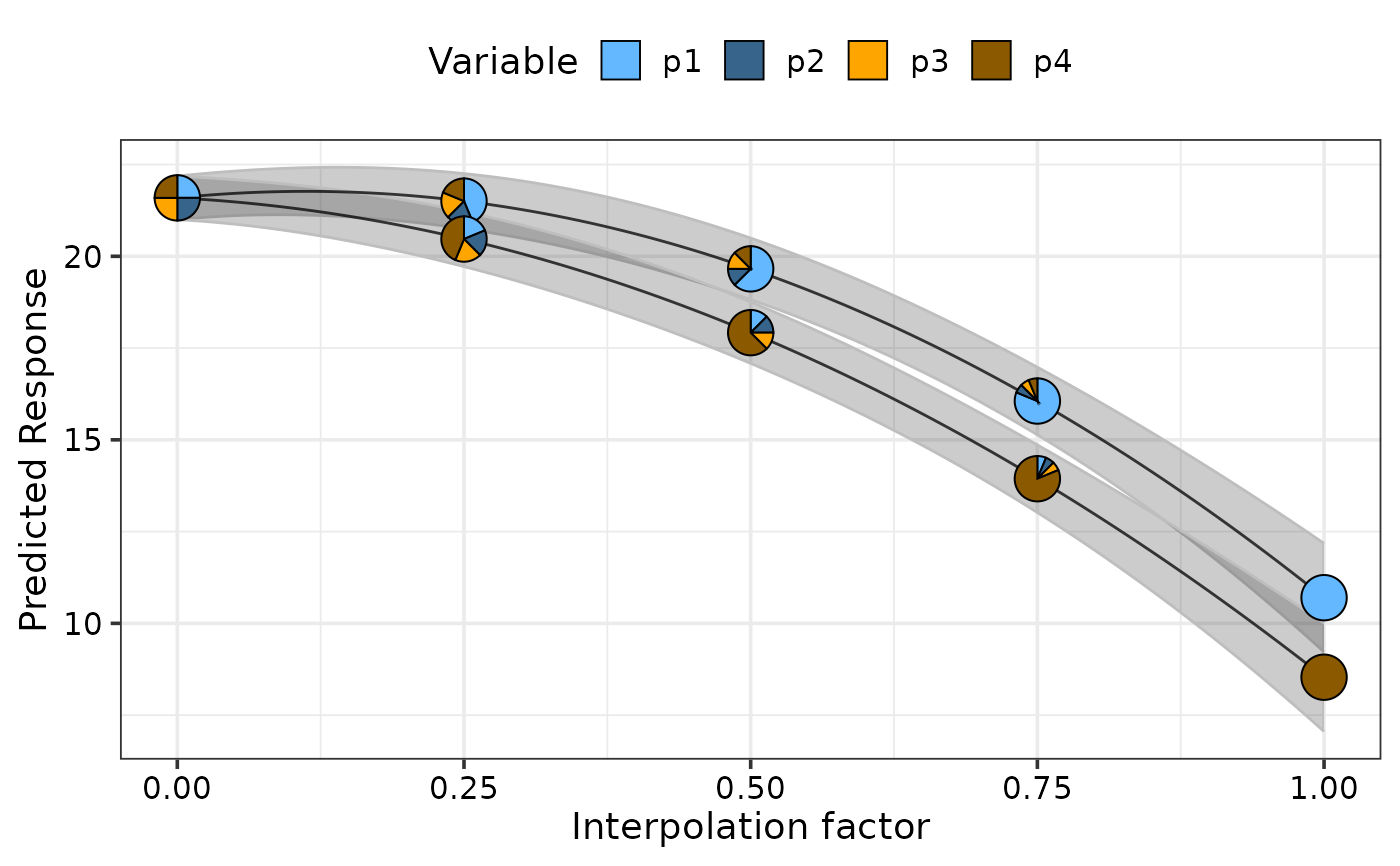
pie_positions: A numeric vector with values between 0 and 1 (both inclusive) indicating the positions along the X-axis at which to show pie-glyphs for each curve. Default is c(0, 0.5, 1) meaning that pie-glyphs with be shown at the start, midpoint and end of each curve.
pie_radius: A numeric value specifying the radius (in cm) for the pie-glyphs. Default is 0.3 cm.
pie_colours: A character vector indicating the colours for the slices in the pie-glyphs.
If left NULL, the colour blind friendly colours will be for the pie-glyph slices.
se: A boolean variable indicating whether to plot confidence intervals associated with the effect of species increase or decrease
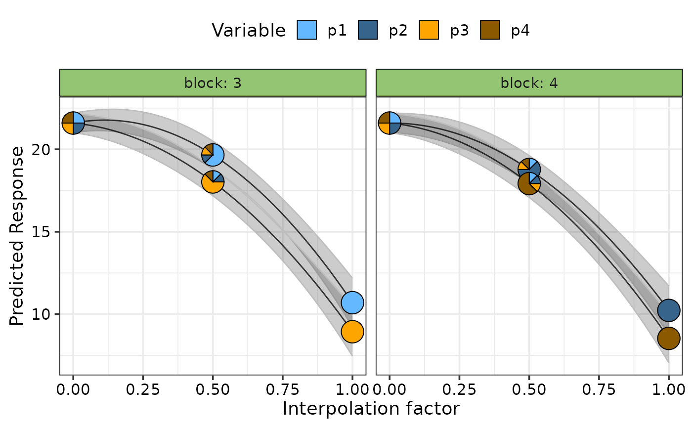
facet_var: A character string or numeric index identifying the column in the data to be used for faceting the plot into multiple panels.
nrow: Number of rows in which to arrange the final plot (when `add_var` is specified).
ncol: Number of columns in which to arrange the final plot (when `add_var` is specified).

Value

A ggmultiplot (ggplot if single plot is returned) class object or data-frame (if `plot = FALSE`)

Examples

library(DImodels)

## Load data
data(sim2)

## Fit model
mod <- glm(response ~ (p1 + p2 + p3 + p4)^2 + 0, data = sim2)

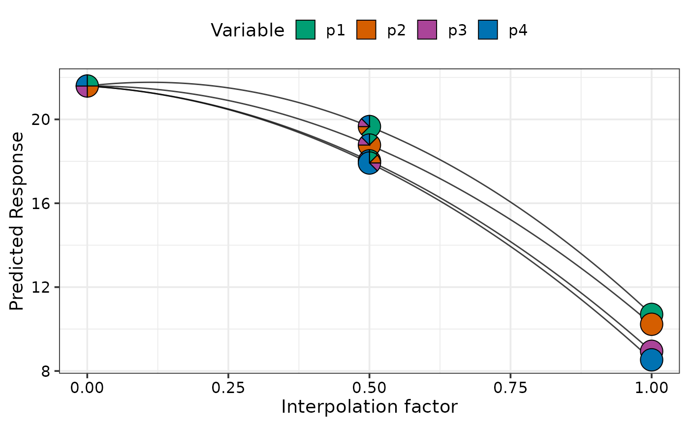
## Visualise change as we move from the centroid community to each monoculture
plot_data <- simplex_path_data(starts = sim2[c(19, 20, 19, 20), ],
                               ends = sim2[c(47, 52, 55, 60), ],
                               prop = c("p1", "p2", "p3", "p4"),
                               model = mod)
#> ✔ Finished data preparation.
## prop will be inferred from data
simplex_path_plot(data = plot_data)
#> ✔ Created plot.


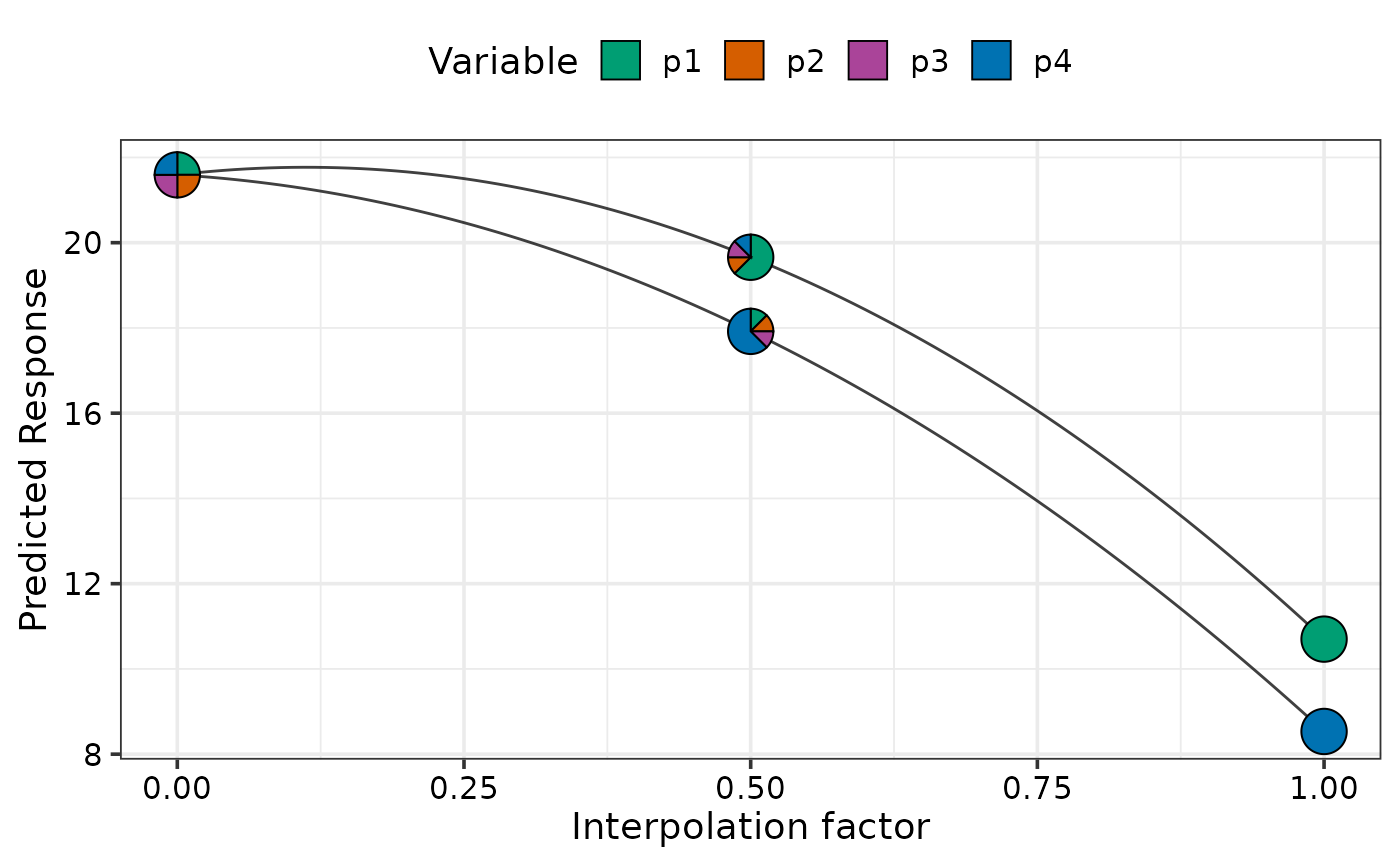
## Show specific curves
simplex_path_plot(data = plot_data[plot_data$.Group %in% c(1, 4), ])
#> ✔ Created plot.


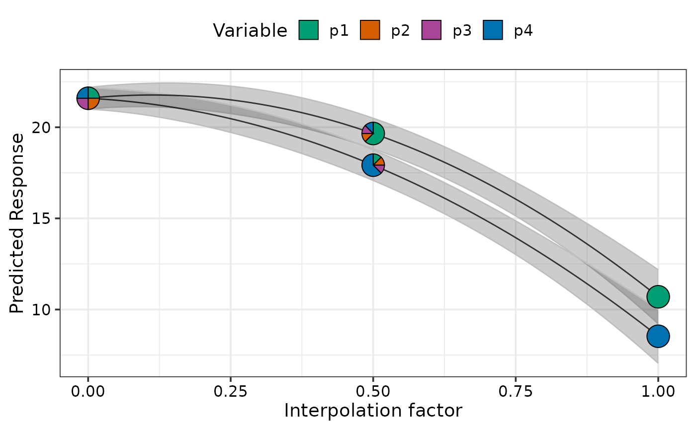
## Show uncertainty using `se = TRUE`
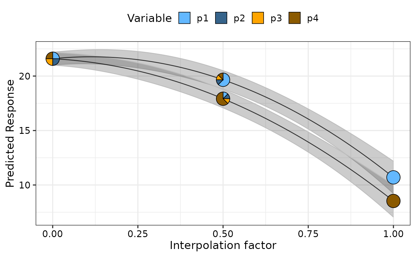
simplex_path_plot(data = plot_data[plot_data$.Group %in% c(1, 4), ],
                  se = TRUE)
#> ✔ Created plot.


## Change colours of pie-glyphs using `pie_colours`
simplex_path_plot(data = plot_data[plot_data$.Group %in% c(1, 4), ],
                  se = TRUE,
                  pie_colours = c("steelblue1", "steelblue4", "orange1", "orange4"))
#> ✔ Created plot.


## Show pie-glyphs at different points along the curve using `pie_positions`
simplex_path_plot(data = plot_data[plot_data$.Group %in% c(1, 4), ],
                  se = TRUE,
                  pie_positions = c(0, 0.25, 0.5, 0.75, 1),
                  pie_colours = c("steelblue1", "steelblue4", "orange1", "orange4"))
#> ✔ Created plot.


## Facet plot based on specific variables
simplex_path_plot(data = plot_data,
                  se = TRUE,
                  facet_var = "block",
                  pie_colours = c("steelblue1", "steelblue4", "orange1", "orange4"))
#> ✔ Created plot.


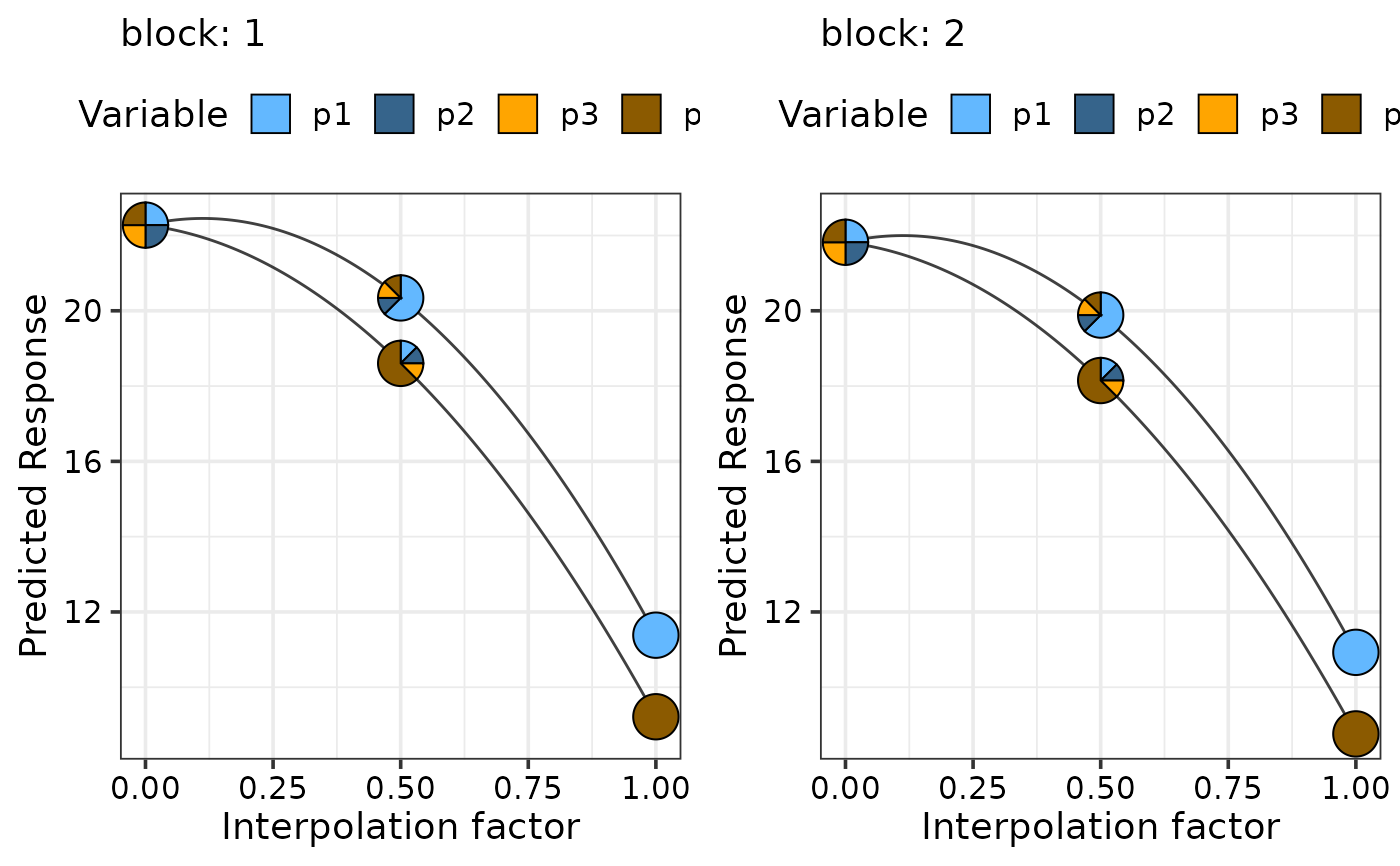
## Simulataneously create multiple plots for additional variables
sim2$block <- as.numeric(sim2$block)
new_mod <- update(mod, ~ . + block, data = sim2)
plot_data <- simplex_path_data(starts = sim2[c(18), 3:6],
                       ends = sim2[c(48, 60), 3:6],
                       prop = c("p1", "p2", "p3", "p4"),
                       model = new_mod, conf.level = 0.95,
                       add_var = list("block" = c(1, 2)))
#> ✔ Finished data preparation.

simplex_path_plot(data = plot_data,
                  pie_colours = c("steelblue1", "steelblue4",
                                  "orange1", "orange4"),
                  nrow = 1, ncol = 2)
#> ✔ Created all plots.