Regression diagnostics plots with pie-glyphs — model

This function returns regression diagnostics plots for a model with points replaced by pie-glyphs making it easier to track various data points in the plots. This could be useful in models with compositional predictors to quickly identify any observations with unusual residuals, hat values, etc.

Usage

model_diagnostics(
  model,
  which = c(1, 2, 3, 5),
  prop = NULL,
  FG = NULL,
  npoints = 3,
  cook_levels = c(0.5, 1),
  pie_radius = 0.2,
  pie_colours = NULL,
  only_extremes = FALSE,
  label_size = 4,
  points_size = 3,
  plot = TRUE,
  nrow = 0,
  ncol = 0
)

Arguments

model: A statistical regression model object fit using lm, glm, nlme functions, etc.
which: A subset of the numbers 1 to 6, by default 1, 2, 3, and 5, referring to
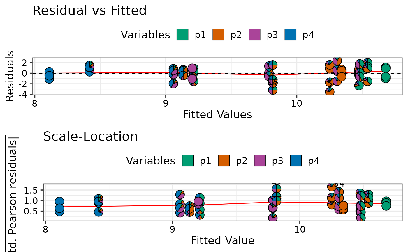
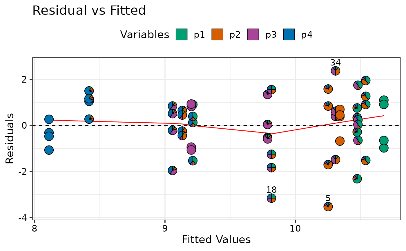
1 - "Residuals vs Fitted", aka "Tukey-Anscombe" plot
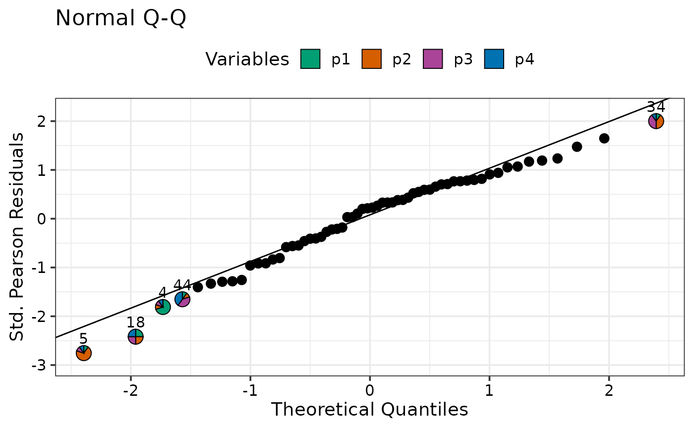
2 - "Normal Q-Q" plot, an enhanced qqnorm(resid(.))
3 - "Scale-Location"
4 - "Cook's distance"
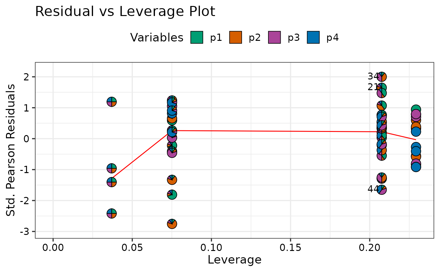
5 - "Residuals vs Leverage"
6 - "Cook's dist vs Lev./(1-Lev.)"
Note: If the specified model object does not inherit the lm class, it might not be possible to create all diagnostics plots. In these cases, the user will be notified about any plots which can't be created.
prop: A character vector giving names of columns containing proportions to show in the pie-glyphs. If not specified, black points (geom_point) will be shown for each observation in the model. Note: \code{prop} can be left blank and will be interpreted if model is a Diversity-Interactions (DI) model object fit using the DI() function from the DImodels package.
FG: A character vector of same length as prop specifying the group each variable belongs to.
npoints: Number of points to be labelled in each plot, starting with the most extreme (those points with the highest absolute residuals or hat values).
cook_levels: A numeric vector specifying levels of Cook's distance at which to draw contours.
pie_radius: A numeric value specifying the radius (in cm) for the pie-glyphs.
pie_colours: A character vector specifying the colours for the slices within the pie-glyphs.
only_extremes: A logical value indicating whether to show pie-glyphs only for extreme observations (points with the highest absolute residuals or hat values).
label_size: A numeric value specifying the size of the labels identifying extreme observations.
points_size: A numeric value specifying the size of points (when pie-glyphs not shown) shown in the plots.
plot: A boolean variable indicating whether to create the plot or return the prepared data instead. The default TRUE creates the plot while FALSE would return the prepared data for plotting. Could be useful if user wants to modify the data first and then create the plot.
nrow: Number of rows in which to arrange the final plot.
ncol: Number of columns in which to arrange the final plot.

Value

A ggmultiplot (ggplot if single plot is returned) class object or data-frame (if plot = FALSE).

Examples

library(DImodels)

## Load data
data(sim1)

## Fit model
mod1 <- lm(response ~ 0 + (p1 + p2 + p3 + p4)^2, data = sim1)

## Get diagnostics plot
## Recommend to store plot in a variable, to access individual plots later
diagnostics <- model_diagnostics(mod1, prop = c("p1", "p2", "p3", "p4"))
#> ✔ Created all plots.
print(diagnostics)


## Access individual plots
print(diagnostics[[1]])

print(diagnostics[[4]])


## Change plot arrangement
# \donttest{
model_diagnostics(mod1, prop = c("p1", "p2", "p3", "p4"),
                  which = c(1, 3), nrow = 2, ncol = 1)
#> ✔ Created all plots.

# }

## Show only extreme points as pie-glyphs to avoid overplotting
model_diagnostics(mod1, prop = c("p1", "p2", "p3", "p4"),
                  which = 2, npoints = 5, only_extremes = TRUE)
#> ✔ Created all plots.


## If model is a DImodels object, the don't need to specify prop
DI_mod <- DI(y = "response", prop = c("p1", "p2", "p3", "p4"),
             DImodel = "FULL", data = sim1)
#> Fitted model: Separate pairwise interactions 'FULL' DImodel
model_diagnostics(DI_mod, which = 1)
#> ✔ Created all plots.


## Specify `plot = FALSE` to not create the plot but return the prepared data
head(model_diagnostics(DI_mod, which = 1, plot  = FALSE))
#>   response p1_ID p2_ID p3_ID p4_ID p1:p2 p1:p3 p1:p4 p2:p3 p2:p4 p3:p4  p1  p2
#> 1   10.815   0.7   0.1   0.1   0.1  0.07  0.07  0.07  0.01  0.01  0.01 0.7 0.1
#> 2   11.232   0.7   0.1   0.1   0.1  0.07  0.07  0.07  0.01  0.01  0.01 0.7 0.1
#> 3   10.192   0.7   0.1   0.1   0.1  0.07  0.07  0.07  0.01  0.01  0.01 0.7 0.1
#> 4    8.157   0.7   0.1   0.1   0.1  0.07  0.07  0.07  0.01  0.01  0.01 0.7 0.1
#> 5    6.724   0.1   0.7   0.1   0.1  0.07  0.01  0.01  0.07  0.07  0.01 0.1 0.7
#> 6   11.093   0.1   0.7   0.1   0.1  0.07  0.01  0.01  0.07  0.07  0.01 0.1 0.7
#>    p3  p4       .hat   .sigma      .cooksd  .fitted     .resid  .stdresid Obs
#> 1 0.1 0.1 0.07512992 1.343832 0.0005750445 10.47436  0.3406361  0.2660631   1
#> 2 0.1 0.1 0.07512992 1.340067 0.0028447324 10.47436  0.7576361  0.5917723   2
#> 3 0.1 0.1 0.07512992 1.344130 0.0003951286 10.47436 -0.2823639 -0.2205480   3
#> 4 0.1 0.1 0.07512992 1.299979 0.0266139030 10.47436 -2.3173639 -1.8100401   4
#> 5 0.1 0.1 0.07512992 1.238479 0.0616767948 10.25177 -3.5277748 -2.7554644   5
#> 6 0.1 0.1 0.07512992 1.338966 0.0035070720 10.25177  0.8412252  0.6570619   6
#>   Label         .qq weights
#> 1     1  0.06270678       1
#> 2     2  0.45376219       1
#> 3     3 -0.31863936       1
#> 4     4 -1.73166440       1
#> 5     5 -2.39397980       1
#> 6     6  0.54852228       1