DI specific wrapper for conditional ternary diagrams
conditional_ternary.RdWe fix \(n-3\) variables to have a constant value \(p_1, p_2, p_3, ... p_{n-3}\)
such that \(P = p_1 + p_2 + p_3 + ... p_{n - 3}\) and \(0 \le P \le 1\) and
vary the proportion of the remaining three variables between \(0\) and \(1-P\)
to visualise the change in the predicted response as a contour map within a
ternary diagram. This is equivalent to taking multiple 2-d slices of the
high dimensional simplex space. Taking multiple 2-d slices across multiple
variables should allow to create an approximation of how the response varies
across the n-dimensional simplex.
This is a wrapper function specifically for statistical models fit using the
DI() function from the
DImodels R package and would implicitly
call conditional_ternary_data followed by
conditional_ternary_plot. If your model object isn't fit using
DImodels, consider calling these functions manually.
Usage
conditional_ternary(
  model,
  FG = NULL,
  values = NULL,
  tern_vars = NULL,
  conditional = NULL,
  add_var = list(),
  resolution = 3,
  plot = TRUE,
  nlevels = 7,
  colours = NULL,
  lower_lim = NULL,
  upper_lim = NULL,
  contour_text = FALSE,
  show_axis_labels = TRUE,
  show_axis_guides = FALSE,
  scale_ternaries = FALSE,
  axis_label_size = 4,
  vertex_label_size = 5,
  nrow = 0,
  ncol = 0
)
Arguments
- model
A Diversity Interactions model object fit by using the
DI()function from theDImodelspackage.- FG
A character vector specifying the grouping of the variables specified in `prop`. Specifying this parameter would call the grouped_ternary_data function internally. See
grouped_ternaryorgrouped_ternary_datafor more information.- values
A numeric vector specifying the proportional split of the variables within a group. The default is to split the group proportion equally between each variable in the group.
- tern_vars
A character vector giving the names of the three variables to be shown in the ternary diagram.
- conditional
A data-frame describing the names of the compositional variables and their respective values at which to slice the simplex space. The format should be, for example, as follows:
data.frame("p1" = c(0, 0.5), "p2" = c(0.2, 0.1))
One figure would be created for each row in `conditional` with the respective values of all specified variables. Any compositional variables not specified in `conditional` will be assumed to be 0.- add_var
A list or data-frame specifying values for additional variables in the model other than the proportions (i.e. not part of the simplex design). This could be useful for comparing the predictions across different values for a non-compositional variable. If specified as a list, it will be expanded to show a plot for each unique combination of values specified, while if specified as a data-frame, one plot would be generated for each row in the data.
- resolution
A number between 1 and 10 describing the resolution of the resultant graph. A high value would result in a higher definition figure but at the cost of being computationally expensive.
- plot
A boolean variable indicating whether to create the plot or return the prepared data instead. The default
TRUEcreates the plot whileFALSEwould return the prepared data for plotting. Could be useful if user wants to modify the data first and then create the plot.- nlevels
The number of levels to show on the contour map.
- colours
A character vector or function specifying the colours for the contour map or points. The number of colours should be same as `nlevels` if (`show = "contours"`).
The default colours scheme is theterrain.colors()for continuous variables and an extended version of the Okabe-Ito colour scale for categorical variables.- lower_lim
A number to set a custom lower limit for the contour (if `show = "contours"`). The default is minimum of the prediction.
- upper_lim
A number to set a custom upper limit for the contour (if `show = "contours"`). The default is maximum of the prediction.
- contour_text
A boolean value indicating whether to include labels on the contour lines showing their values (if `show = "contours"`). The default is
FALSE.- show_axis_labels
A boolean value indicating whether to show axis labels along the edges of the ternary. The default is
TRUE.- show_axis_guides
A boolean value indicating whether to show axis guides within the interior of the ternary. The default is
FALSE.- scale_ternaries
Accepts boolean values. If TRUE, each ternary is scaled by \(1 - P\), where \(P\) is the sum of the conditioning proportions and \(0 \le P \le 1\). Note that ternaries may become very small when `P` is close to 1. Default is FALSE.
- axis_label_size
A numeric value to adjust the size of the axis labels in the ternary plot. The default size is 4.
- vertex_label_size
A numeric value to adjust the size of the vertex labels in the ternary plot. The default size is 5.
- nrow
Number of rows in which to arrange the final plot (when `add_var` is specified).
- ncol
Number of columns in which to arrange the final plot (when `add_var` is specified).
Value
A ggmultiplot (ggplot if single plot is returned) class object or data-frame (if `plot = FALSE`)
Examples
library(DImodels)
library(dplyr)
#>
#> Attaching package: ‘dplyr’
#> The following objects are masked from ‘package:stats’:
#>
#> filter, lag
#> The following objects are masked from ‘package:base’:
#>
#> intersect, setdiff, setequal, union
data(sim2)
m1 <- DI(y = "response", data = sim2, prop = 3:6, DImodel = "FULL")
#> Fitted model: Separate pairwise interactions 'FULL' DImodel
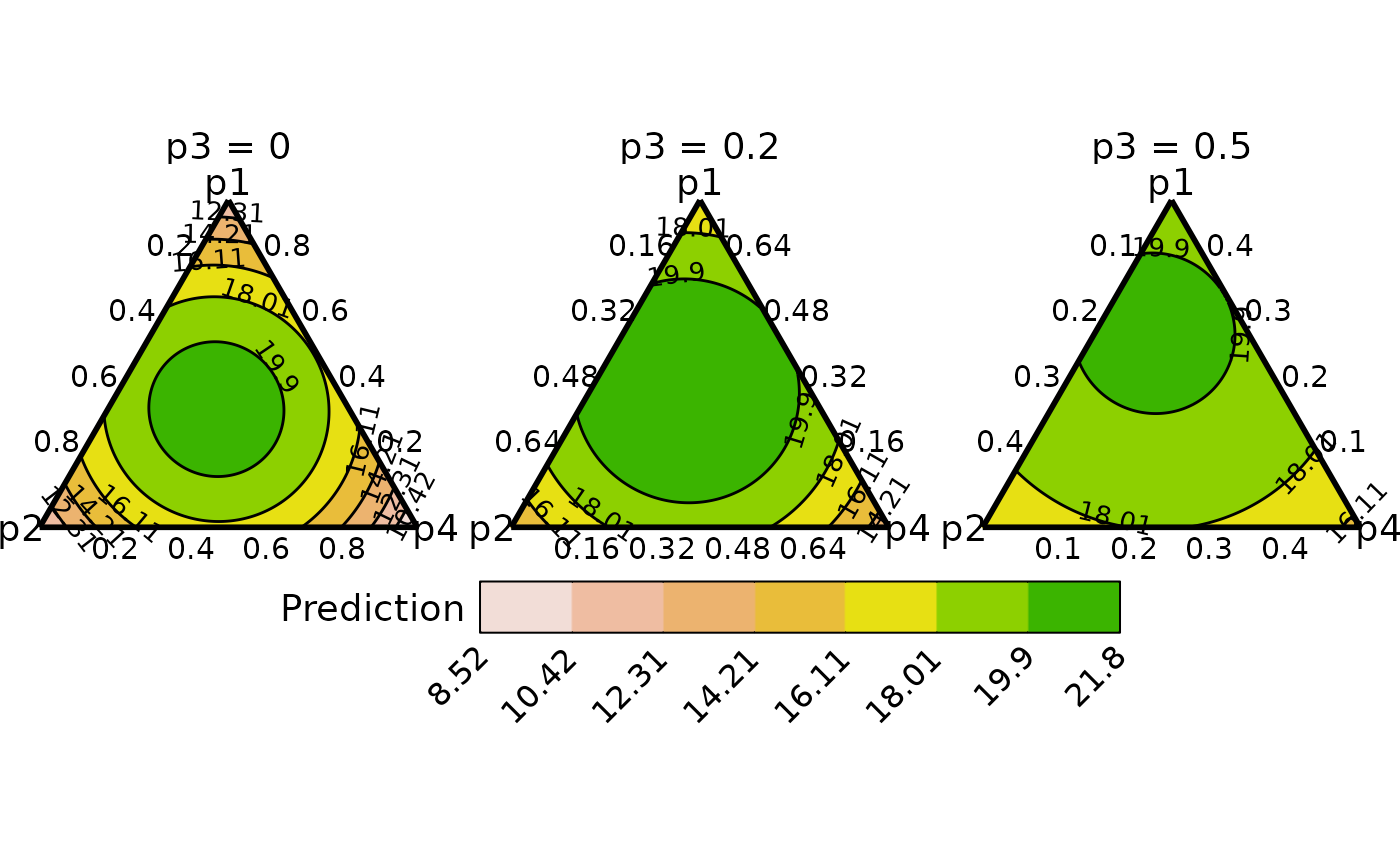
## We only condition on the variable "p3"
conditional_ternary(model = m1, tern_vars = c("p1", "p2", "p4"),
conditional = data.frame("p3" = c(0, 0.2, 0.5)),
resolution = 1)
#> ✔ Finished data preparation.
#> ✔ Created plot.
 ## Allow ternary size to scale based on value of conditioning variable
conditional_ternary(model = m1, tern_vars = c("p1", "p2", "p4"),
conditional = data.frame("p3" = c(0, 0.2, 0.5)),
resolution = 1, scale_ternaries = TRUE)
#> ✔ Finished data preparation.
#> ✔ Created plot.
## Allow ternary size to scale based on value of conditioning variable
conditional_ternary(model = m1, tern_vars = c("p1", "p2", "p4"),
conditional = data.frame("p3" = c(0, 0.2, 0.5)),
resolution = 1, scale_ternaries = TRUE)
#> ✔ Finished data preparation.
#> ✔ Created plot.
 ## Slices for experiments for over 4 variables
data(sim4)
m2 <- DI(y = "response", prop = paste0("p", 1:6),
DImodel = "AV", data = sim4) %>%
suppressWarnings()
#> Fitted model: Average interactions 'AV' DImodel
## Conditioning on multiple variables
cond <- data.frame(p4 = c(0, 0.2), p3 = c(0.5, 0.1), p6 = c(0, 0.3))
conditional_ternary(model = m2, conditional = cond,
tern_vars = c("p1", "p2", "p5"), resolution = 1)
#> ✔ Finished data preparation.
#> ✔ Created plot.
## Slices for experiments for over 4 variables
data(sim4)
m2 <- DI(y = "response", prop = paste0("p", 1:6),
DImodel = "AV", data = sim4) %>%
suppressWarnings()
#> Fitted model: Average interactions 'AV' DImodel
## Conditioning on multiple variables
cond <- data.frame(p4 = c(0, 0.2), p3 = c(0.5, 0.1), p6 = c(0, 0.3))
conditional_ternary(model = m2, conditional = cond,
tern_vars = c("p1", "p2", "p5"), resolution = 1)
#> ✔ Finished data preparation.
#> ✔ Created plot.
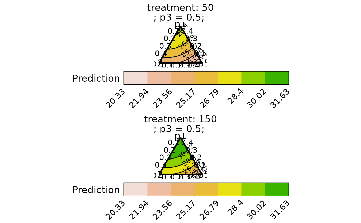 ## Create separate plots for additional variables not a part of the simplex
m3 <- DI(y = "response", prop = paste0("p", 1:6),
DImodel = "AV", data = sim4, treat = "treatment") %>%
suppressWarnings()
#> Fitted model: Average interactions 'AV' DImodel
## Create plot and arrange it using nrow and ncol
# \donttest{
conditional_ternary(model = m3, conditional = cond[1, ],
tern_vars = c("p1", "p2", "p5"),
resolution = 1,
add_var = list("treatment" = c(50, 150)),
nrow = 2, ncol = 1)
#> ✔ Finished data preparation.
#> ✔ Created all plots.
## Create separate plots for additional variables not a part of the simplex
m3 <- DI(y = "response", prop = paste0("p", 1:6),
DImodel = "AV", data = sim4, treat = "treatment") %>%
suppressWarnings()
#> Fitted model: Average interactions 'AV' DImodel
## Create plot and arrange it using nrow and ncol
# \donttest{
conditional_ternary(model = m3, conditional = cond[1, ],
tern_vars = c("p1", "p2", "p5"),
resolution = 1,
add_var = list("treatment" = c(50, 150)),
nrow = 2, ncol = 1)
#> ✔ Finished data preparation.
#> ✔ Created all plots.
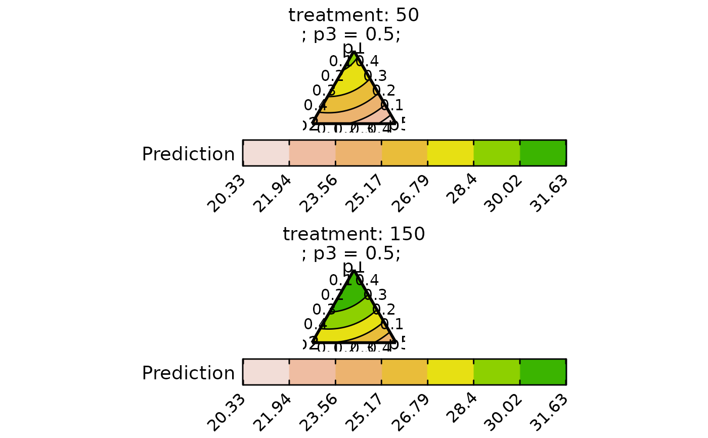 # }
## Specify `plot = FALSE` to not create the plot but return the prepared data
head(conditional_ternary(model = m3, conditional = cond[1, ],
resolution = 1, plot = FALSE,
tern_vars = c("p1", "p2", "p5"),
add_var = list("treatment" = c(50, 150))))
#> ✔ Finished data preparation.
#> p1 p2 p5 .x .y p4 p3 p6 treatment .add_str_ID
#> 1 0 0.5000000 0.000000000 0.000000000 0 0 0.5 0 50 treatment: 50
#> 2 0 0.4974874 0.002512563 0.005025126 0 0 0.5 0 50 treatment: 50
#> 3 0 0.4949749 0.005025126 0.010050251 0 0 0.5 0 50 treatment: 50
#> 4 0 0.4924623 0.007537688 0.015075377 0 0 0.5 0 50 treatment: 50
#> 5 0 0.4899497 0.010050251 0.020100503 0 0 0.5 0 50 treatment: 50
#> 6 0 0.4874372 0.012562814 0.025125628 0 0 0.5 0 50 treatment: 50
#> .Sp .Value .Facet .Pred
#> 1 p4, p3, p6 0, 0.5, 0 p4 = 0; p3 = 0.5; p6 = 0 23.64637
#> 2 p4, p3, p6 0, 0.5, 0 p4 = 0; p3 = 0.5; p6 = 0 23.65679
#> 3 p4, p3, p6 0, 0.5, 0 p4 = 0; p3 = 0.5; p6 = 0 23.66693
#> 4 p4, p3, p6 0, 0.5, 0 p4 = 0; p3 = 0.5; p6 = 0 23.67680
#> 5 p4, p3, p6 0, 0.5, 0 p4 = 0; p3 = 0.5; p6 = 0 23.68639
#> 6 p4, p3, p6 0, 0.5, 0 p4 = 0; p3 = 0.5; p6 = 0 23.69572
# }
## Specify `plot = FALSE` to not create the plot but return the prepared data
head(conditional_ternary(model = m3, conditional = cond[1, ],
resolution = 1, plot = FALSE,
tern_vars = c("p1", "p2", "p5"),
add_var = list("treatment" = c(50, 150))))
#> ✔ Finished data preparation.
#> p1 p2 p5 .x .y p4 p3 p6 treatment .add_str_ID
#> 1 0 0.5000000 0.000000000 0.000000000 0 0 0.5 0 50 treatment: 50
#> 2 0 0.4974874 0.002512563 0.005025126 0 0 0.5 0 50 treatment: 50
#> 3 0 0.4949749 0.005025126 0.010050251 0 0 0.5 0 50 treatment: 50
#> 4 0 0.4924623 0.007537688 0.015075377 0 0 0.5 0 50 treatment: 50
#> 5 0 0.4899497 0.010050251 0.020100503 0 0 0.5 0 50 treatment: 50
#> 6 0 0.4874372 0.012562814 0.025125628 0 0 0.5 0 50 treatment: 50
#> .Sp .Value .Facet .Pred
#> 1 p4, p3, p6 0, 0.5, 0 p4 = 0; p3 = 0.5; p6 = 0 23.64637
#> 2 p4, p3, p6 0, 0.5, 0 p4 = 0; p3 = 0.5; p6 = 0 23.65679
#> 3 p4, p3, p6 0, 0.5, 0 p4 = 0; p3 = 0.5; p6 = 0 23.66693
#> 4 p4, p3, p6 0, 0.5, 0 p4 = 0; p3 = 0.5; p6 = 0 23.67680
#> 5 p4, p3, p6 0, 0.5, 0 p4 = 0; p3 = 0.5; p6 = 0 23.68639
#> 6 p4, p3, p6 0, 0.5, 0 p4 = 0; p3 = 0.5; p6 = 0 23.69572